Difference between revisions of "Contrib:KeesWouters/staticshell"
Keeswouters (Talk | contribs) (→'''General remarks with respect to element selection''') |
Keeswouters (Talk | contribs) (→'''General remarks with respect to element selection''') |
||
| Line 93: | Line 93: | ||
* in linear statics, prefer quadratic elements | * in linear statics, prefer quadratic elements | ||
* for large strain / plasticity, try both and look which one is best | * for large strain / plasticity, try both and look which one is best | ||
| − | (there are no really pathologic elements in 2D) | + | * (there are no really pathologic elements in 2D) |
I hope that it will help you in your analysis - Joël''' | I hope that it will help you in your analysis - Joël''' | ||
Revision as of 10:16, 20 May 2009
Contents
Static behaviour of rectangular plate
The dynamics of a rectangular plate can be predicted quite well with shell (coque_3d) elements. I also liked to know the accuracy of the displacements for this kind of structures. A comparison between solid elements and shell elements has been made.
Dimensions of the plate
The length and width of the plate are 1*1 m. The thickness of the shell elements has been increased to 0.02 m to enable meshing with solid elements (tetrahedrons and hexahedrons).
Boundary conditions and load
Two types of boundary conditions will be discussed:
- clamped at one side (all displacements and rotations are suppressed)
- [clamped at the four sides, tbd]
The load on the structure is a pressure of 0.1 bar on the surface of the plate.
Material properties
The Young's module and poisson ratio for steel are set to 210 GPa and 0.28.
Displacement at the tip using beam theory
According to the shell theory the displacement of a beam the tip under uniform pressure is:
- w = q*L^4/(8*D)
- uniform pressure q = 10 kPa
- length of plate L = 1 m
- Youngs' module E = 210 GPa
- poisson ratio nu = 0.28
- bending stiffness D = Eh^3/(12*(1-nu*nu)) = 151910 Nm and
- displacement at the tip w = 8.2286 mm
Salome model of the rectangular plate
Shell elements
The geometry and meshing follows the same procedure as for the dynamics: geometry of the plate and generating the mesh.
For a full description on shells see e.g Code Aster documentation (coque_3d).
Boundary conditions
For these calculations all the degree of freedoms (dofs) on one edge of the plate have been suppressed: three displacements and three rotations. This has been done in the corresponding comm file with the following rule:
clamped=AFFE_CHAR_MECA(MODELE=modelc,
                       DDL_IMPO=(_F(GROUP_MA=('Linex0',),
                                   DX=0.0,
                                   DY=0.0,
                                   DZ=0.0,
                                   DRX=0.0,
                                   DRY=0.0,
                                   DRZ=0.0,),),
                        FORCE_COQUE=_F(GROUP_MA='shell',
                                   PRES=10.0e3,),);
The group Linex0, of course, defines one edge of the plate. The applied load FORCE_COQUE defines a surface load or pressure of 10 kPa on the group 'shell'.
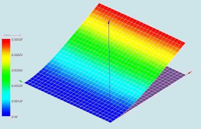
For this load case the calculated displacement at the tip of the plate is
w_ca = 8.460 mm for a mesh with 40 nodes (3*3 quad8/9 elements) and
w_ca = 8.473 mm for a mesh with 2300 nodes.
In both cases this is slightly more than the theoretical value based on the shell theory: +2.8 % and +3.0 % for 40 and 2300 nodes respectively.
Comparison of displacement to solid elements
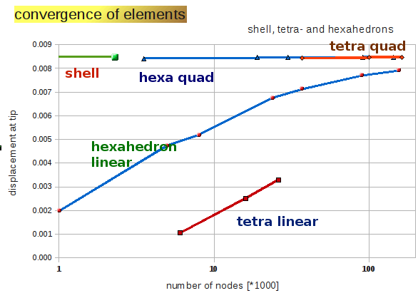
So it may be noted that the shell elements converge fairly rapidly to the correct value. We expect that for solid elements convergence will be much slower.
In the graph below the results of some calculations are shown. We have used tetrahedron and hexahedron elements, both linear and quadratic.
On the x-axis the number of nodes (thousands of nodes) are given. They range from 40 for the shell mesh to nearly 150k for the solid elements. On the vertical axis the calculated displacement is given where the convergence value is about 0.0085 m.
Note that the 150k nodes is about the maximum my hardware is able to handle. It needs about 3.5 GB ram for this calculation and my physical limit is 4 GB now.
So it is fair to say that linear elements will be much too stiff for normal cases. Therefor the displacements of the structure will be predicted much too low. There has been a discussion about this many times on the CAElinux forums, but I didnot expect that linear elements give such a large stiffness compared to quadratic elements.
General remarks with respect to element selection
From the graph it is clear that we should use quadratic elements as much as possible. Here Joël Cugnoni makes the following, more general statements:
Concerning the choice of element / mesh refinement, here is a summary of my recommendations:
For 3D stress analysis in linear statics without contact:
- use quadratic elements by default: they will give you systematically better results than linear elements
- completely forget the linear tetrahedron, they are always too stiff and give bad stress predictions, their convergence rate is also very low (error does not change much if you refine the mesh)
- if you need to use linear elements: only use hexa or prisms. When bending is significant, put at least 2-4 linear elements through the thickness. To avoid "locking": try to keep the element aspect ratio between 1 and 5 or use reduced elements
For 3D stress analysis in non-linear statics & contact:
- in large strain analysis (plasticity), the enhanced accuracy of quadratic elements is usually less significant than in linear statics. The non-linear geometric effects and integration of local constitutive behaviour are more important. In this sense tetra are not the best choice in this case (strange plastic strain localization patterns...) My advice is to try several meshes and different element types (and exact/reduced integration). For highly non-linear studies, the best choice usually is a nice structured hexahedric mesh (linear or quadratic depending on the case)
- with contact, quadratic elements tend to have large contact pressure oscillation and may induce solver convergence problems. I would recommend to use a fine linear hexahedric (or at least prisms) mesh in this case
For 2D stress analysis:
- in linear statics, prefer quadratic elements
- for large strain / plasticity, try both and look which one is best
- (there are no really pathologic elements in 2D)
I hope that it will help you in your analysis - Joël
Table of results
The displacement at the tip for various numbers of nodes, number of layers over the thickness and different elements are given in the table below. This table has been used to compose the graph above.
mesh type w_ca Rel % KNodes layers
shell quad 0.008460  102.81   0.04
shell quad 0.008473  102.96   2.3

tetra LIN  0.001049  12.75    6     1
tetra LIN  0.002515  30.57    16    2
tetra LIN  0.003300  40.10    26    2

tetra Quad 0.008423  102.37   37    1
tetra Quad 0.008459  102.81   100   2
tetra Quad 0.008461  102.83   163   2

hexa LIN   0.001984  24.11    1     2
hexa LIN   0.004738  57.58    5     3
hexa LIN   0.005193  63.11    8     4
hexa LIN   0.006756  82.10    24    5
hexa LIN   0.007128  86.62    37    6
hexa LIN   0.007698  93.55    90    8
hexa LIN   0.007911  96.14    156  10
hexa Quad  0.008415  102.26   3.5   2
hexa Quad  0.008450  102.69   19    3
hexa Quad  0.008454  102.74   30    4
hexa Quad  0.008461  102.82   91    5
hexa Quad  0.008462  102.84   143   6
first column:  mesh type: shell, hexahedron, tetrahedron (LINear or Quadratic)
second column: displacement at the tip [m]
third column:  relative displacement at the tip, compared to shell theory
fourth column: number of nodes
fifth column:  number of layer along the thickness
Mesh with solid elements
For comparison solid elements have been used to determine the behaviour of the plate.
It is easy in Salome to change from linear to quadratic elements: in the menu bar in the Mesh Module click on Modification-->Convert to/from quadratic or use the conversion icon on the top right. The you have the choice of converting to/from quadratic depending on the initial situation. Converting from linear to quadratic you also have the choice to place the medium node on the geometry: click the box medium nodes on geometry.
In most cases the calculation has been carried out with linear and quadratic elements using the same mesh grid. Saving the mesh into the med file after conversion is all that needs to be done. Starting the Code Aster calculations by ASTK is just hitting the run button if all file and directories are set.
Boundary conditions for the solid elements
Because the solid elements have no rotational degree of freedom the clamped edges must be given by fixed displacement of the side planes. The boundary conditions and loads are now defined in the comm file by:
clamp1=AFFE_CHAR_MECA(MODELE=ModQuad,
                      DDL_IMPO=(_F(GROUP_MA='f1',
                                   DX=0.0,
                                   DY=0.0,
                                   DZ=0.0,),),
                    PRES_REP=_F(GROUP_MA='surfbot',
                                   PRES=10000.0,),);
The group f1 is one of the side planes of the plate and all displacements on it are suppressed by the DDL_IMPO statement. The group 'surfbot' are all the shell elements.
The complete command file is given here: Media:commandfile.comm.zip
Hexahedron elements
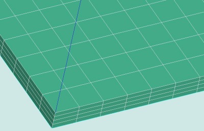
The following python file defines the geometry and the mesh of the plate. The mesh consists of hexahedron elements. The number of nodes and elements is largely controlled by the parameter Mfineness at the start of the file. Set this value to 0.15 and it yields exactly 30k nodes. The number of layer along the thickness of the plate is 4. Setting different values for Mfineness (in the range from 0.0 to 0.6) yields between 2 and 12 layers. For large number of nodes only linear elements can be solved due to lack of memory on my hardware.
Media:geom_mesh_solidplate.zip
mesh with Hexahedron elements
Tetrahedron elements
Now change the meshing part in the python file to:
elemVol = 0.12
TMesh = smesh.Mesh(Extrusion1)
Tetrahedron_Netgen = TMesh.Tetrahedron(algo=smesh.NETGEN)
Max_Element_Volume = Tetrahedron_Netgen.MaxElementVolume(elemVol)
Max_Element_Volume.SetMaxElementVolume(elemVol)
smeshObj = smesh.smesh.CreateHypothesis('NETGEN_Parameters_2D','NETGENEngine')
Netgen_1D_2D = smesh.smesh.CreateHypothesis('NETGEN_2D','NETGENEngine')
status = TMesh.AddHypothesis(Netgen_1D_2D)
isDone = TMesh.Compute()
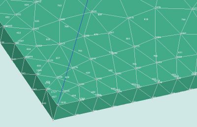
which basicly set the Netgen 3D and 2D parameters with the parameter elemVol. Setting elemVol=0.12 yields a linear mesh with 1.8k nodes with only one layer along the height of the plate, see picture.
mesh with tetrahedron elements
The stresses in the plate - hexahedron elements
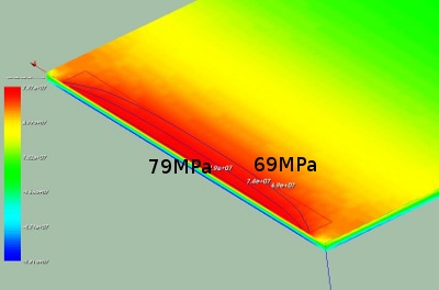
Using the solid elements it is easy to determine the relevant stresses in the plate. In the next picture the stress sigma_yy at the bottom of the plate (the group surfbot in the Salome definition) are depicted. According to the theory this stress should be |sigma_yy| = 3*q/b*(L/h)^2 = 75 MPa. In the calculation the stresses go up to nearly 80 MPa.
The stresses in the plate - shell elements
Depending on which layer you would like to have the stresses, you need to define in the command file:
* for layer NIVE_COUCHE='SUP' (superieur, top)
* for layer NIVE_COUCHE='MOY' (moyenne, center)
* for layer NIVE_COUCHE='INF' (inferieur, bottom)
e.g to define the stresses in the top layer you can use the following sequence of commands:
# define top layer by 'SUP'
top=CALC_ELEM(REPE_COQUE=_F(NUME_COUCHE=1,NIVE_COUCHE='SUP',),
             OPTION=('SIGM_ELNO_DEPL','EQUI_ELNO_SIGM',),
             RESULTAT=result,);
 ....
 top=CALC_NO(reuse=top,
           RESULTAT=top,
           OPTION='SIGM_NOEU_DEPL',);
 ...
 # because Salome has a different mesh (quad8 iso coque_3d/quad9) we have to recalculate the stress fields to the initial Salome mesh
 salomT=PROJ_CHAMP(RESULTAT=top,
                   MODELE_1=modelc,    # project fields of this model to
                   MODELE_2=modinit,); # field of model_2
 ...
 # and finally print the results.
 # stresses in ['SUP', salomT, top], ['MOY', salomC, centre] and ['INF', salomB, bottom] layer,
 # displacements in salomR
 IMPR_RESU(FORMAT='MED',
         UNITE=21,
         RESU=(_F(MAILLAGE=meshinit,RESULTAT=salomT,
                  NOM_CHAM=('SIGM_NOEU_DEPL','EQUI_NOEU_SIGM','EQUI_ELNO_SIGM','DEPL','SIGM_ELNO_COQU',),),
               _F(MAILLAGE=meshinit,RESULTAT=salomB,
                  NOM_CHAM=('SIGM_NOEU_DEPL','EQUI_NOEU_SIGM','EQUI_ELNO_SIGM','DEPL','SIGM_ELNO_COQU',),),
               _F(MAILLAGE=meshinit,RESULTAT=salomC,
                  NOM_CHAM=('SIGM_NOEU_DEPL','EQUI_NOEU_SIGM','EQUI_ELNO_SIGM','DEPL','SIGM_ELNO_COQU',),),
               _F(MAILLAGE=meshinit,RESULTAT=salomR,
                  NOM_CHAM=('SIGM_NOEU_DEPL','EQUI_NOEU_SIGM','EQUI_ELNO_SIGM','DEPL','SIGM_ELNO_COQU',),),),);
So also discussion here: http://www.code-aster.org/forum2/viewtopic.php?id=12523, help from, amoung others, Johannes Ackva and Thomas de Soza much appreciated.
The full command file is here: Media:kw_shell22.comm.zip
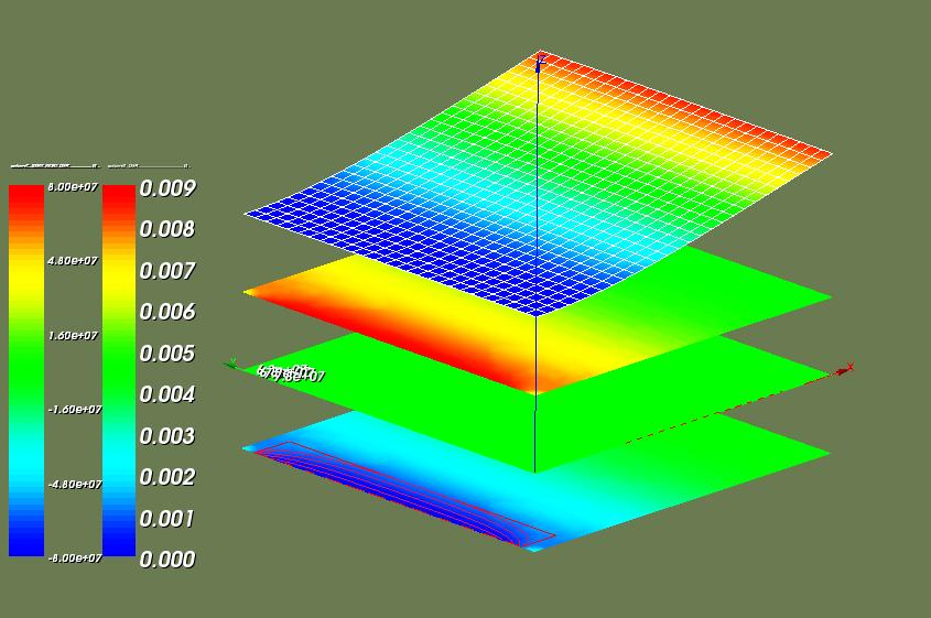
In the picture below the stresses are given in the three layers (bottom three fields). The displacement is given at the top.
In Salome a shift in z direction is given:
 +0.4 for the displacement field.
 +0.2 for top stresses,
  0.0 for centre stresses,
 -0.2 for bottom stresses,
The first legend in the picture indicates the stress, the second indicates the displacement in z direction.
Again the maximum absolute stress here is |sigma_xx| = 79 MPa, the same value that has been found by the hexahedron elements.
Remarks - notes - to do:
* [The labels of the stress values do not shift with the field somehow, so the values given in the centre layer belong to the bottom]
* [I am not sure whether all specified fields in the definition of the stresses are relevant/correct ('SIGM_NOEU_DEPL','EQUI_NOEU_SIGM',
'EQUI_ELNO_SIGM','DEPL','SIGM_ELNO_COQU',), I do not have a complete overview of the exact meaning of every keyword. So if anybody is willing to give an update or link here, pls do]
* [still need to figure out to indicate the normal vector of each element, although this also may be pretty obvious.]
--kwarky 14:44, 7 May 2009 (CEST)
