Contrib:KeesWouters/plate/thickness
Contents
- 1 Varying thickness of shells - by Python
- 2 Extraction of the coordinates
- 3 General - extraction of coordinates
- 4 Things that might go wrong
- 5 Post processing with Salome
- 6 Total mass of the plate
- 7 Input and output files for the FE Analysis
- 8 CODE ASTER version 10.X - TRIA6_7 and QUAD8_9
- 9 References
Varying thickness of shells - by Python
Static displacement of a shell under pressure
november 2010 - SalomeMeca 2010 (Code Aster 10.2) - Ubuntu Meerkat 10.10 64bits.
This is just a simple example of the use of shells (coque_3d) for static calculations. The main focus is on varying thickness of the shell by a Python list. The thickness of the shell depends on the average Ycog coordinate of the shell element.
General way of determination of the shell thickness
First the geometry and mesh is generated in Salome in the standard way. In Code Aster the mesh is read, including nodes number, node coordinates, element types and element connectivity. We use quadratic quad8 elements that are converted to quad9 (coque_3d) elements suitable for C Aster. Of each element the nodes are determined by the connectivity matrix, the coordinates of all the nodes and finally the centre of gravity. This includes the y coordinate Ycog. The element thickness th is calculated by th = Ycog*0.1+0.01 and stored in a Python list. This list is passed to the AFFE_CARA_ELEM command. Further processing C Aster is from then on as usual.
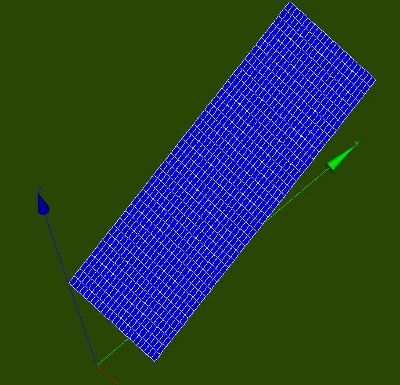
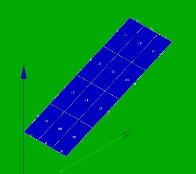
Geometry, mesh and material properties
The construction is a rectangle in the xyz plane. Minimum x is 0, maximum x is 1.0 [m]. For y and z these values are: [ymin, ymax] = [0.0, 2.5] and [zmin, zmax] = [1.25, 2.3456]. The varying thickness of the plate depends on the average y coordinate as follows: th = Ycog*0.1+0.01.
Boundary conditions are as follows: the two edges parallel to the y axis are restricted in all six directions. The material is steel, its mechanical properties are defined by the following parameters: Young's modulus E = 2.1e11 Pa, poisson ratio NU=0.28 [-] and density -though not needed- here RHO=7850 kg/m3. For more details see e.g. here where the details of the general calculation procedure are given. In the next part we concentrate on the extraction of the coordinates of the elements and the definition of the thickness of each element.
Extraction of the coordinates
Among others, in this Code Aster forum this procedure is discussed.
In Code Aster, after reading the initial mesh, the quad8 elements are converted to quad9 (coque_3d compatible) elements. This mesh is called meshmod (modified mesh) and is used as the basis for the further operations.
First we adapt the DEBUT() command since we need real Python commands:
DEBUT(PAR_LOT='NON');
We import the partition module in the command file to read mesh quantities. And the complete definition of the thickness of the shells is stored in a separate Python script/module/file (construct_shell_thickness) in the path defined below:
from Utilitai.partition import *
import sys
sys.path.append('/cae/caexample/shell/shellplate_thlist')
from construct_shell_thickness import *
After reading the initial mesh meshinit with quad8 elements
meshinit=LIRE_MAILLAGE(FORMAT='MED',INFO=1,);
and converting it to quad9, coque_3d elements
meshmod=CREA_MAILLAGE(MAILLAGE=meshinit,
                     MODI_MAILLE=(_F(TOUT='OUI',
                                     OPTION='QUAD8_9',),),);
we define the local thickness of each element by calling
info = 1
ThicknessGroupShell = construct_shell_thickness(meshmod,info)
The Python script construct_shell_thickness does the whole trick. Have a look at this in detail. Standard, the characteristics of the shell are defined by the AFFE_CARA_ELEM command with, among others, the following parameters:
shellch=AFFE_CARA_ELEM(MODELE=modmod,
                      COQUE=_F(GROUP_MA='shell',
                               EPAIS=0.001,),);
Now remember that the parameters in the _F(...) operator can be replaced by Pyhton list, in this case: ellist = {'GROUP_MA': 'shell','EPAIS':0.001}. Or more general:
 ellist = [{'MAILLE': 'Mxxx','EPAIS':thxxx},
           {'MAILLE': 'Myyy','EPAIS':thyyy},
           { .......                      },
           { .......                      },
           {'MAILLE': 'Mzzz','EPAIS':thzzz}]
where 'Mxxx' is the element number and thxxx is the corresponding element thickness. Eg in this example the following list is generated:
thicknessGroupShell:
[{'EPAIS': 0.15423076923076928, 'MAILLE': 'M127'},
 {'EPAIS': 0.21192307692307708, 'MAILLE': 'M128'},
 .....
 {'EPAIS': 0.15423076923076931, 'MAILLE': 'M1061'},
 {'EPAIS': 0.21192307692307702, 'MAILLE': 'M1062'}]
General - extraction of coordinates
The actual thickness of the shell depends on the average y coordinate of it. This is extracted as follows. First read the mesh and extract a new mesh by the commands
meshCA   = MAIL_PY()
meshCA.FromAster(mesh)
In meshCA all the quantities can be extracted:
 nonu     = meshCA.dime_maillage[0]    ## number of nodes
 elnu     = meshCA.dime_maillage[2]    ## number of elements
 ncoord   = meshCA.cn                  ## coordinates of the nodes
 connect  = meshCA.co                  ## connectivity of the element
 NodeList = list(meshCA.correspondance_noeuds)   ## says it all
 ElemList = list(meshCA.correspondance_mailles)
 ElemType = list(meshCA.tm)
The procedure is then as follows:
- step through element list
- check if element type is quad9/coque_3d/number 16
- read connectivity of the element: connectivity = meshCA.co
- step through all node of the element
- determine nodes and its coordinates
- compute average (y) coordinate
- define thickness depending on (y) coordinate
- add thickness and element to list {...}
In 'real' Python code:
for ii in xrange(len(ElemList)):
  print ElemType[ii]
  if ElemType[ii]==16:  # select shell (coque_3d) elements
    #print connect[ii]
    shellcount +=1
ThicknessGroupShell=[]
thickness = [None]*shellcount
shellcount = 0
for ii in xrange(len(ElemList)):
  print 'elementtype: ',ii,ElemType[ii]
  if ElemType[ii]==16:  # select shell coque_3d elements 14:quad8, 16:quad9
    sumxyz = [0.0, 0.0, 0.0]
    ncount = len(connect[ii])    # should be 9 for coque_3d (elementType 16)
    for jj in xrange(0,ncount):
      Gnode = connect[ii][jj]    # globalnode = connect[elemii,internal_nodejj]
      sumxyz += ncoord[Gnode]    # this might be written more compact --> for later
    sumxyz /=ncount
    # define your own code for thickness here
    # thickness now depends on average y coordinate only
    thickness[shellcount] = sumxyz[1]*0.1+0.01  # make thickness depent on y coordinate
    tempth = thickness[shellcount]
    shellcount +=1
    #print 'average xyz - centre point: ',sumxyz,ncoord[Gnode]  #centre point is same average nodes
    ThicknessGroupShell.append({'EPAIS':tempth,'MAILLE':'M%d'%(ii+1)});  ## add 1 for element number Mxx
Normally, vecteur or angle??? and NCOU ??? need to be defined as well. Now the trick is
Things that might go wrong
Of course, nothing will ever go wrong. Except code written in Python and used in conjunction with Code Aster of course. All things go wrong then. First all kind of syntax error occur. These are relatively easy to capture and remove, because Python normally offers help by issuing nice error messages. Things are less trivial if you forget the +1 to inidicate the mesh element in the append command: 'MAILLE':'M%d'%(ii+1) because of the different numbering of Salome and Code Aster mesh (I guess). To see how the mesh is built up you can print the whole mesh FromAster: print meshCA, meshCA = MAIL_PY(), meshCA.FromAster(mesh).
Then you get eg:
COOR_3D
N1         1.00000000000000E+00   2.50000000000000E+00   2.34560000000000E+00
....
SEG3
M1        N3       N17      N18
....
QUAD9
M15       N10      N29      N30      N12      N36      N37      N38
      N13      NS1
....
GROUP_MA
Linex0
M5       M7       M10      M11
FINSF
%
GROUP_MA
Linex1
M3       M9       M12      M14
FINSF
%
GROUP_MA
shell
M15      M16      M17      M18      M19      M20      M21      M22
M23      M24      M25      M26
This allows you to check the correct node numbers, elements, connectivity and groups defined in your mesh. Starting with a small mesh is advicable.
Also carefully check the code that generates the thickness of the shell. It is very easy to make a mistake: selecting the wrong index of the coordinate array is an obvious one.
For a small mesh (3 by 4 elements) the Python list is as follows:
thicknessGroupShell:
[{'EPAIS': 0.16625000000000001, 'MAILLE': 'M15'},
 {'EPAIS': 0.22875000000000001, 'MAILLE': 'M16'},
 {'EPAIS': 0.041250000000000002, 'MAILLE': 'M17'},
 {'EPAIS': 0.22875000000000001, 'MAILLE': 'M18'},
 {'EPAIS': 0.16625000000000001, 'MAILLE': 'M19'},
 {'EPAIS': 0.10375, 'MAILLE': 'M20'},
 {'EPAIS': 0.10375, 'MAILLE': 'M21'},
 {'EPAIS': 0.041250000000000002, 'MAILLE': 'M22'},
 {'EPAIS': 0.041250000000000002, 'MAILLE': 'M23'},
 {'EPAIS': 0.16625000000000001, 'MAILLE': 'M24'},
 {'EPAIS': 0.22875000000000001, 'MAILLE': 'M25'},
 {'EPAIS': 0.10375, 'MAILLE': 'M26'}]
# define BC and loads
# for all the edges of the plate the z displacement is fixed [DZ=0.0]
# one edge [Linex0] is kept fixed in y direction [DY=0.0] and
# another edge [Liney0] is kept fixed in x direction [DX=0.0]
Loaddyn=AFFE_CHAR_MECA(MODELE=modmod,
                      DDL_IMPO=(_F(GROUP_MA='Linex0',
                                   DY=0.0,
                                   DZ=0.0,),
                                _F(GROUP_MA='Liney0',
                                   DX=0.0,
                                   DZ=0.0,),
                                _F(GROUP_MA=('Liney1','Linex1',),
                                   DZ=0.0,),),);
# define the calculation
# determine stiffness and mass matrix depending on material, mesh and applied  model (coque_3D) for dynamic calculation (mode shapes and frequencies)
MACRO_MATR_ASSE(MODELE=modmod,
               CHAM_MATER=material,
               CARA_ELEM=shellch,
               CHARGE=Loaddyn,
               NUME_DDL=CO('NUMEDDL'),
               MATR_ASSE=(_F(MATRICE=CO('RIGIDITE'),
                             OPTION='RIGI_MECA',),
                          _F(MATRICE=CO('MASSE'),
                             OPTION='MASS_MECA',),),);
# determine the frequencies within the band 1 and 50 Hz
MODES=MODE_ITER_SIMULT(MATR_A=RIGIDITE,
                      MATR_B=MASSE,
                      CALC_FREQ=_F(OPTION='BANDE',
                                   FREQ=(1.0,50.0,),),);
# determine / project the result fields (champ) from modified model modmod to the initial model modinit
salomres=PROJ_CHAMP(RESULTAT=MODES,
                   MODELE_1=modmod,      #project modes/results of model_1
                   MODELE_2=modinit,);   #to model_2
# store the results in a MED file
# only the displacements 'DEPL' will be stored
# note that UNITe 21 corresponds to the LU column of ASTK.
IMPR_RESU(FORMAT='MED',
         UNITE=80,
         RESU=_F(MAILLAGE=meshinit,
                 RESULTAT=MODES,
                 NOM_CHAM='DEPL',),);
#fin
FIN();
The comm file (see end of this contributionn) may be edited by Eficas [under Tools --> Command file editor (Eficas)] in the ASTK menu bar. You get a number of possible entries for each command.
Post processing with Salome
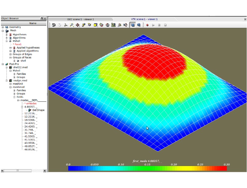
Return back to Salome, select Post Pro and select by File --> Import --> res33.med ie. the result file defined by ASTK (res33.med). Now the nice part of the work starts by making some colourful pictures. In the left window click on Post Pro and the + res33 appears. Click onthe plus (+) sign and the two meshes appear: meshinit and meshmod. Each have some subfields. The most interesting is the field Fields in meshmod. Click again on the + in front of the Fields and the frequencies of the MODES___DEPL___ appear. Now right click on the + sign in front of one of the frequencies and play around with the settings of the template window and modes shapes appear in the VTK viewer window. Have fun with different setting, by right clicking on the Def.Shape field below the frequency.
A view of the first mode shape is given here:
Comparison to analytic results
All four boundaries of the plate are hinged. Comparing the first five analytic (Fth) to the numerical (Fnum) results [Hz] and relative differences, gives the following table:
 shape       Fth        Fnum         dif %
 1*1       7.429       7.425        -0.054
 1*2      14.757      14.751        -0.041
 2*1      22.389      22.381        -0.036
 1*3      26.974      26.963        -0.041
 2*2      29.715      29.702        -0.044
In total 8 eigenvalues are present in the range below 50 Hz, from 7 to is 47 Hz. The analytical results are according to G.B. Warburton, the vibration of rectangular plates, 1954.
Total mass of the plate
Finally we add a command to determine the mass of the shell. At the end of the command file add the following lines:
masshell=POST_ELEM(MASS_INER=_F(GROUP_MA='shell',),
                  MODELE=modmod,
                  CHAM_MATER=material,
                  CARA_ELEM=shellch,);
IMPR_TABLE(TABLE=masshell,NOM_PARA='MASSE',);
FIN();
The results are written to a table in the resu file, in this case the shell33.resu.med file.
#ASTER  9.04.06 CONCEPT masshell CALCULE LE 14/05/2009 A 11:54:43 DE TYPE
#TABLE_SDASTER
 MASSE
  7.85000E+00
Standard the tables are written to unite 8, the result file. To write to a seperate file, add a line in ASTK with type 'resu', filename ./masse.txt (in Linux) and unit number (LU) e.g. 22, change the command line into:
IMPR_TABLE(TABLE=masshell,UNITE=22,NOM_PARA='MASSE',);
and the results are nicely written to the file masse.txt seperately from all messages in the result file.
[You can also get the centre of gravity and the inertia of the construction, but I did succeed in doing that.]
Input and output files for the FE Analysis
Input files:
- Python script for defining the geometry (geom_plate1by1.py)
- Python script for defining the mesh (mesh_plate1by1.py)
- python script of geometry and mesh (combination of those above, geom_mesh_plate1by1.py)
- ASTK file (shelldyn.astk, you need to edit the path to your requirements ...)
- command file (shelldyn.comm)
output file:
- total mass returned by CA (masse.txt)
download the files here:
- >>>Media:Fea_plate1by1.zip: error on TRIA6_7 in Code Aster10, please do not use anymore
- >>>Media: kw_platedyn_ca10.zip: suitable for Aster10
CODE ASTER version 10.X - TRIA6_7 and QUAD8_9
Update in the second version:
shellch=AFFE_CARA_ELEM(MODELE=modmod,
                      COQUE=_F(GROUP_MA='shell',
                               EPAIS=th,
                               COQUE_NCOU=1,),);
meshmod=CREA_MAILLAGE(MAILLAGE=meshinit,
                     MODI_MAILLE=(_F(TOUT='OUI',OPTION='QUAD8_9',),),);
CREA_MAILLAGE
The problem is that no TRIA6 elements are present in the mesh. So
version Fea_plate1by1.zip works on Code-Aster 9.xx but not on version 10.xx.
In this example only Quad8 elements are present. The MODI_MAILLAGE keyword in the CREA_MAILLAGE comnmand in C-Aster 10 does not accept this part: _F(TOUT='OUI',OPTION='TRIA6_7',) anymore.
....MODI_MAILLE=(_F(TOUT='OUI',OPTION='QUAD8_9',),
                 _F(TOUT='OUI',OPTION='TRIA6_7',),) ....;
If both TRIA6 and QUAD8 elements are present use:
meshmod=CREA_MAILLAGE(MAILLAGE=meshinit,
                      MODI_MAILLE=(_F(TOUT='OUI',OPTION='QUAD8_9',),
                                   _F(TOUT='OUI',OPTION='TRIA6_7',),),);
If only QUAD8 elements (quadrangles) are available use:
meshmod=CREA_MAILLAGE(MAILLAGE=meshinit,
                      MODI_MAILLE=(_F(TOUT='OUI',OPTION='QUAD8_9',),),);
If only TRIA6 elements (triangles) are available use:
meshmod=CREA_MAILLAGE(MAILLAGE=meshinit,
                      MODI_MAILLE=(_F(TOUT='OUI',OPTION='TRIA6_7',),),);
The message file reports QUAD8 elements not available, but I guess it it the absence of TRIA6 elements that causes a F_COPY_ERROR:
MOT CLE FACTEUR "MODI_MAILLE", OCCURRENCE    1
 MODIFICATION DE    729 MAILLES    QUAD8 EN    QUAD9
! <EXCEPTION> <MODELISA3_32>                               !
!  Erreur utilisateur dans CREA_MAILLAGE/MODI_MAILLE :     !
!   Vous avez demandé la transformation de type QUAD8_9.   !
!   Mais il n'y a aucune maille quadratique à transformer. !
References
From Code Aster references:
[u2.02.01] Notice d’utilisation des éléments plaques, coques et coques volumiques SHB
[u4.81.22] Opérateur POST_ELEM
[u5.02.00] Manuel d’Utilisation - Fascicule U5.0- : Structure de données resultat Document: U5.02.00 - Présentation des tables
[u3.12.03] Modélisation COQUE_3D
[R3.07.04] Eléments finis de coques volumiques
[R3.07.05] Éléments de coques volumiques en non linéaire
géométrique
Overview of units - Paul Carrico
--keeswouters 17:11, 24 April 2009 (CEST)


