Contrib:Claws/Real world study CodeSaturne
Contents
Real world study with Code Saturne
Content
Introduction
For a long time I've wanted to try and use CFD for a practical purpose and compare it to real-world results, and now during my internship, I have the chance to try it out. For all intent and purposes, I'm far from an expert on CFD nor fluid dynamics, but I have done a few experiments and have a good general idea of how things come together in fluid dynamics/CFD. What this sums up to, is 'nothing is written in stone here' – There may be errors and the setup is probably far from optimal, there is always room for improvement.
- Here is a hands on case with Code Saturne without getting too technical.
Goal
To create a computer model that corresponds to real world – with the goal of further development of burner tube. This is an initial simulation to make sure I can make Code_Saturne emulate real world conditions. The goal is however, not to be 100% physically correct, nor does time permit me to set up the experiment to a laboratory grade.
Scenario
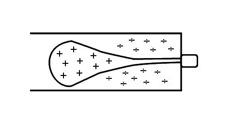
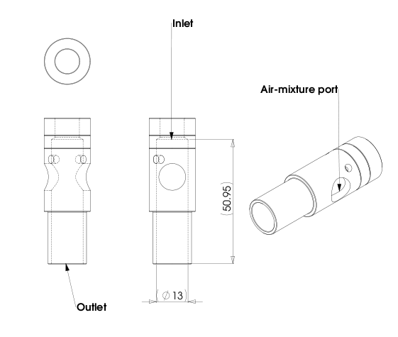
In a gas fire a burner tube is used to mix the fuel (in this case natural gas) with oxygen using the Venturi effect. The pressurized fuel is sent from the high pressure bottle, through a regulator and from the regulator through a nozzle into the burner tube. The gas jet from the nozzle creates a low pressure zone around the base of the jet which sucks in air through the aeration port and mixes it in the burner tube before it is sent into the burner1.
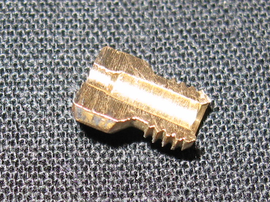
Among other things, the geometry of the nozzle and the velocity of the fluid determines the shape of the jet and the magnitude of the low pressure zone. In this case I've guestimated a discharge coefficient of 0.5, based on the geometry of the nozzle and calculated the exit velocity accordingly.
The exit orifice has a diameter of ~1.9mm
In this study I wont simulate what happens inside the nozzle, nor will I concern myself too much whether the shape of the gas jet is physically correct at the exit – That will be discussed a bit more later on.
Mathematical approach
Collecting data
For my simulation I need to input some data into the model, this was done in the following manner:
- Measure volumetric flow rate of the gas going into the burner tube using a flow-meter on the actual gas fire and compare it to the technical documents specified by the test lab
- Guestimate a discharge coefficient for the nozzle using empirical numbers from a table
- Acquiring physical properties for natural gas (using pure methane)
- Measure pressure differential on the regulator
- Calculate exit velocity of gas jet using above values
Result
Calculating the exit velocity at the nozzle has been done in two ways – using the flow rate and using a theoretical approach. Both results equals ~38m/s but since I know that that is a bit high considering the setup and the values used, I back it down a bit to ~33m/s for the simulation.
See Media:Mathcad-dyse.xmcd.pdf MathCAD PDF for calculation.
Simulation approach
Software
- SolidWorks for modeling the flow domain
- Salomé 4.1.4 for preparing geometry and meshing flow domain
- Code Saturne 1.4b for solving the simulation
- Paraview 3.4.0 for Post processing
Everything besides SolidWorks is run on Ubuntu 8.10 Linux – SolidWorks could easily be replaced by Salomé but laziness dictated I did it in SW at work.
The computer used is my trusty Zepto Znote 6014W, 1.7ghz Celeron, 1GB RAM
Model description and preparation
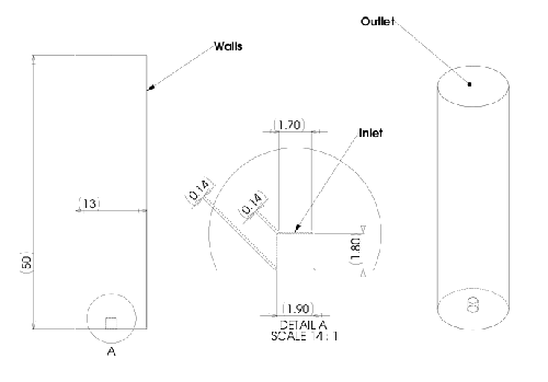
The simplified flow domain consists of a cylinder (Ø13mm, h 50mm) with a simplified inlet (remember, I don't care too much about what happens near and around the inlet).
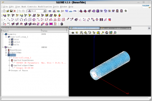
This is exported from SolidWorks in STEP file format and assigned groups in Salomé geometry module, before it is meshed in the meshing module using the following parameters:
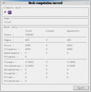
- NetGen 1D-2D-3D using the setting 'very fine' and 'quadratic' (2nd order) – the NetGen algorithm and geometry makes sure that the mesh is refined around the inlet and coarsens further up the flow domain.
This yields the following mesh:
Again, without getting too technical, a way to make sure your mesh is optimized for the simulation, you can calculate the Courant number and adjust your mesh accordingly. ((u*deltat)/deltax)<C
Preparing and running simulation
The mesh is exported in MED file format to the folder ~/Study/MESH/ and the Saturne GUI is started from ~/Study/CASE1/DATA/ using ./SaturneGUI
Code Saturne GUI
Once the GUI has loaded, it is time to enter the values (the options/tabs not mentioned is left at default if nothing is stated).
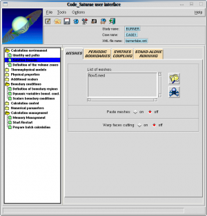
Under Solution domain load the mesh file exported from Salomé :
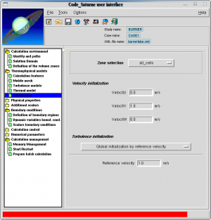
Next go into Thermophysical models and set the turbulence model to k-epsilon – This is a high Renolds number model since that's what I have here.
Initialization is set as seen here:
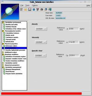
Next the physical properties of the fluid needs to be set:
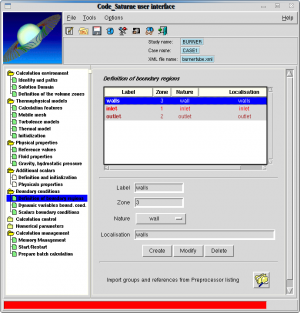
Definition of boundary regions are set next – the names of the boundary regions corresponds to the group names assigned in Salomé.
Entering the calculated velocity in the positive Y-direction in Dynamic variables bound. cond.
Since this is a steady state condition, this is what I left it at in Steady Management.
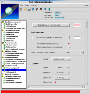
Under Output control I set it to Post-processing every 'n' time step to 1 and select Ensight Gold as the output format (This is so ParaView can post-process the result):
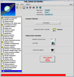
Once everything is set up, theres only one thing left: Load the 'runcase' file under Prepare batch calculation and press Code Saturne batch running:
This launches the calculation and outputs the temporary results in ~/tmp_saturne and the finished results in ~/Study/CASE1/RESU
As the calculation runs, issueing the terminal command
tail -qf ~/tmp_saturne/Study.CASE1.date/listing
will give info on the progress and convergence of the calculation:
INSTANT 0.220000000E+03 TIME STEP NUMBER 220
=============================================================
** BOUNDARY MASS FLOW INFORMATION
------------------------------
Phase : 1
---------------------------------------------------------------
Boundary type Code Nb faces Mass flow
---------------------------------------------------------------
Entree 2 349 -0.489401493E+02
Paroi lisse 5 5207 0.429746002E-16
Paroi rugueuse 6 0 0.000000000E+00
Symetrie 4 0 0.000000000E+00
Sortie libre 3 136 0.489401492E+02
Indefini 1 0 0.000000000E+00
---------------------------------------------------------------
** BOUNDARY CONDITIONS FOR SMOOTH WALLS
---------------------------------------
------------------------------------------------------------
Phase 1 Minimum Maximum
------------------------------------------------------------
Rel velocity at the wall uiptn : -0.27173E+01 0.84489E+01
Friction velocity uet : 0.37369E-03 0.43771E+00
Friction velocity uk : 0.54475E-01 0.41828E+01
Dimensionless distance yplus : 0.50161E+02 0.40720E+05
------------------------------------------------------
Nb of reversal of the velocity at the wall : 1
Nb of faces within the viscous sub-layer : 0
Total number of wall faces : 5207
------------------------------------------------------------
Phase 1 incoming flow detained for 31 outlet faces on 136
** INFORMATIONS ON THE CONVERGENCE
-------------------------------
---------------------------------------------------------------
Variable Rhs norm N_iter Norm. residual derive
---------------------------------------------------------------
c Pressure 0.78903E+01 916 0.97950E-08 0.40786E+00
c VelocitU 0.71071E+02 134 0.92046E-08 0.94592E-01
c VelocitV 0.67696E+03 116 0.89371E-08 0.59835E+00
c VelocitW 0.73505E+02 126 0.95992E-08 0.71705E-01
c TurbEner 0.76674E+03 98 0.97515E-08 0.26028E+00
c Dissip 0.58401E+06 42 0.95251E-08 0.32006E+03
---------------------------------------------------------------
** INFORMATIONS ON THE VARIABLES
-----------------------------
---------------------------------------------------------------
Variable Min. value Max. value Min clip Max clip
---------------------------------------------------------------
v Pressure -0.63469E+02 0.28898E+02 -- --
v VelocitU -0.69839E+01 0.82191E+01 -- --
v VelocitV -0.13238E+02 0.37839E+02 -- --
v VelocitW -0.76948E+01 0.82500E+01 -- --
v TurbEner 0.55144E-03 0.87445E+02 0 0
v Dissip 0.63614E-02 0.36588E+05 8 0
v turb. vi 0.53370E-06 0.13664E+01 0 0
v total_pressu 0.10124E+06 0.10133E+06 0 0
---------------------------------------------------------------
** INFORMATIONS ON THE CLIPPINGS
-----------------------------
---------------------------------------------------------------
Variable Min wo clips Max wo clips Min clip Max clip
---------------------------------------------------------------
a TurbEner 0.55144E-03 0.87445E+02 0 0
a Dissip -0.87143E+02 0.36588E+05 8 0
---------------------------------------------------------------
CPU TIME FOR THE TIME STEP 220: 0.43967E+02
***************************************************************
If everything went smoothly, Code_Saturne rewards you with a “Normal Simulation Finished” and one can move on to...
Post processing
Fire up ParaView and select File → open → Study/CASE1/RESU/CHR.ENSIGHT.date/chr.case
Click 'apply' and select Filters → Alphabetical → Cell data to point data and Filters → Common → Slice and de-select show plane select Z Normal – click apply
Cell data to point data will give a much more smooth representation of the fields and allow showing the velocity field as streamlines.
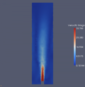
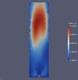
Images are captured at timestep 200 where we have a reasonably steady state:
Pressure:
Media:BurnerTube_pressure.avi.gz
Velocity:
Media:BurnerTube_velocity.avi.gz
Turbulent energy:
Media:BurnerTube_Turbulent_energy.avi.gz
Turbulence – magnitude
Media:BurnerTube_Turbulence.avi.gz
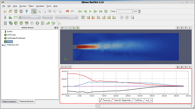
ParaView set up with Plot over line to show values along the X axis:
So after post processing the simulation, what conclusions can be drawn?
Velocity is indeed 33m/s as was the initial condition. The low pressure zone around the base of the jet is ~-22Pa, this is what I'm interested in, since this is what I plan to measure later on in the practical approach. The zones for turbulence and turbulent energy isn't that surprising at all – I'll keep that in mind for when I have to modify the burner tube later on.
Practical approach
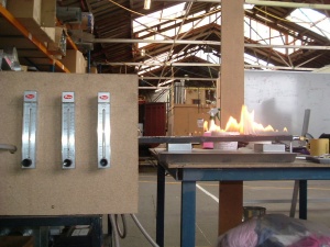
So now I've gotten the simulation to finish and have reasonable derivatives(?), I proceed to do a practical test on the burner tube. First I want to measure the gas flowing into the burner tube; this is done with a flow meter connected between the gas bottle and the regulator. The results of the measurement is used in the MathCAD document both to hold up against the technical document on the gas burner and to control my theoretical calculation.
In this image the middle flowmeter is used and if you squint, you can see the ball hovering at around 6[l/min].
During the run of the flow measurement, I attach a manometer to the low pressure side of the regulator to make sure it has the proper inlet pressure: 1[kPa]
Next up is the actual measurement of the burner tube. I have attached a small fitting to the aeration port and sealed the ports with electrical tape. This should hopefully emulate the simulation setup.
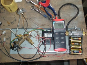
Turning on the gas and letting it flow free through the burner tube with a micro-manometer attached, gave the following reading:
Well how about that! Results are pretty damn close to that of the simulation. Given the circumstances and the setup, a difference of ~3[Pa] is acceptable.
Conclusion
Goal archived, I have a model on which I can build further on.
Code_Saturne can be a harsh mistress. I've have spent many many hours tweaking the shape of the mesh for a seemingly simple numerical analysis. Especially the inlet takes much care to model – the initial 'backlash' of the fluid as it enters the tube (as seen in the animations) has given me much grievance. The trick in this case since I was only interested in low pressures zone in the steady state, was to let the inlet protrude into the chamber to allow for the 'backlashing' – otherwise I got wildly inaccurate if any, results.
CFD requires you to know exactly what you want to retrieve from the simulation and under what conditions. It simply does not converge if you don't have some idea of what mesh size, inlet velocity etc. etc. to apply. This takes much experimentation, at least for me since I don't have a formal background in fluid dynamics.
Don't do CFD on a 1.7ghz celeron if you have the choice – it will wear you out.
File list
Contains STEP of flow volume, .hdf with geo. and mesh and the Code_Saturne .xml file. Media:BURNER.tar.gz
